# usual suspects
library(tidyverse)
library(knitr)
library(fitdistrplus)

# new kid on the block
library(simmer)
library(simmer.plot)
library(simmer.bricks)#5 Queuing using Simmer
14:540:384: Simulation Models in IE (Spring 2025)
Questions
1 Review
- Shown why we need simulations and a few practical examples
- Discussed where distributions come from, how to get them and how to use them
- Shown how to manipulate data and create visualizations
- Demonstrated two coding patterns for simulations
2 Learning Objectives
- Problem analysis
- Set up a simple simulation with
simmer - Run the simulation and extract results
3 Problem
Revisit the Wholefoods Return queue
- customers arrive at a rate \(\lambda = 3/min\)
- single server with exponential service time with \(\mu = 1/2min\)
- run this simulation for 4 hours
4 Implementation
- simmer: a process-oriented and trajectory-based Discrete-Event Simulation (DES) package for R
- Allows us to define the essentials of our system
- It handles the simulation part as well as extracting metrics and nice visualizations
4.1 Loading Packages
4.2 Defining Model
# all given in minutes
lambda <- 1/3
mu <- 1/2
t_f <- 4*60

RV_arr <- function(n=1) {
  rexp(n, rate = lambda)
}

RV_service <- function(n=1) {
  rexp(n, rate = mu)
}
4.3 Simmer Components
Environment: The simulation environment, which contains the resources and processes
Trajectories: The paths that entities take through the simulation, which define the sequence of events that occur
Resources: The resources that are used in the simulation, such as servers, buses, and waiting areas
Let’s break the problem down into components
4.3.1 Customer Trajectory
cust_traj <- trajectory() |>
  seize("clerk", 1) |>
  timeout(function() RV_service(1)) |>
release("clerk", 1)- Very basic trajectory. Customer shows up, gets in line (if necessary), makes a return, and leaves as shown in @plot-customer-trajectory
plot(cust_traj)- some bug I’ll investigate and demonstrate next time how to get the plot to appear correctly.
4.3.2 More complex trajectory
More complex plotted trajectory from the docs
4.3.3 Instantiating the Simulation Environment
return_line <- simmer() |>
  add_resource("clerk", 1) |>
  add_generator("customer", cust_traj, function() RV_arr(1))
4.4 Running the Simulation
return_line |> run(t_f)simmer environment: anonymous | now: 240 | next: 240.785768094172
{ Monitor: in memory }
{ Resource: clerk | monitored: TRUE | server status: 1(1) | queue status: 1(Inf) }
{ Source: customer | monitored: 1 | n_generated: 87 }4.5 Getting Results
get_mon_resources: gets information about the “server” usage get_mon_arrivals: gets information about the “customers”
4.5.1 Resource Visualization
resources <- get_mon_resources(return_line)

kable(head(resources))- averages over time:
plot(resources, metric = "usage")
- instantaneous usage:
plot(resources, metric = "usage", steps=TRUE)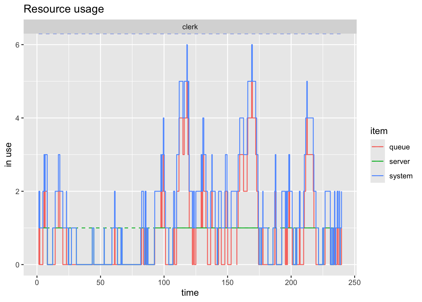
- utiliazation of the resources. Not super interesting here due to only one resource
plot(resources, metric = "utilization")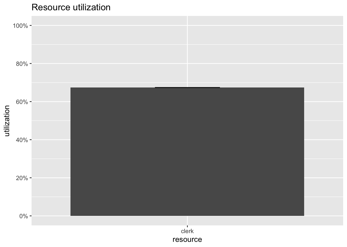
- looking at just the queue
plot(resources, metric = "usage", items="queue", steps=TRUE)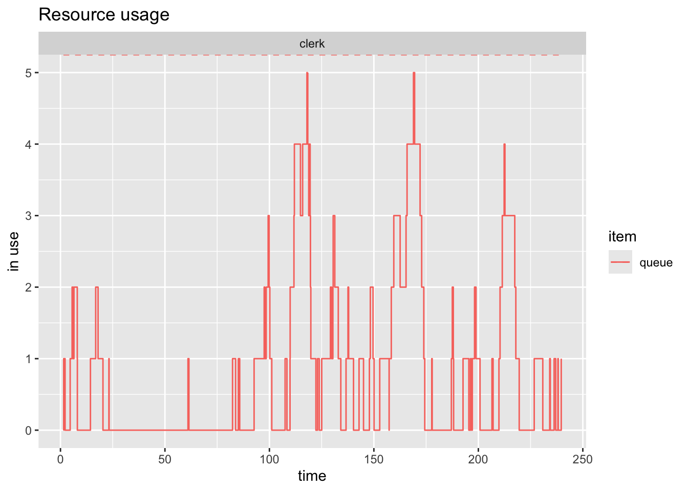
plot(resources, metric = "usage", items="server", steps=TRUE)
4.5.2 Customer Visualization
arrivals <- get_mon_arrivals(return_line)

kable(head(arrivals))| name | start_time | end_time | activity_time | finished | replication |
|---|---|---|---|---|---|
| customer0 | 1.415610 | 2.212143 | 0.7965332 | TRUE | 1 |
| customer1 | 1.537848 | 6.077795 | 3.8656514 | TRUE | 1 |
| customer2 | 4.641538 | 8.041888 | 1.9640935 | TRUE | 1 |
| customer3 | 5.554621 | 8.082859 | 0.0409708 | TRUE | 1 |
| customer4 | 6.454990 | 8.230710 | 0.1478507 | TRUE | 1 |
| customer5 | 12.354493 | 18.001193 | 5.6467005 | TRUE | 1 |
plot(arrivals, metric = "activity_time")`geom_smooth()` using method = 'loess' and formula = 'y ~ x'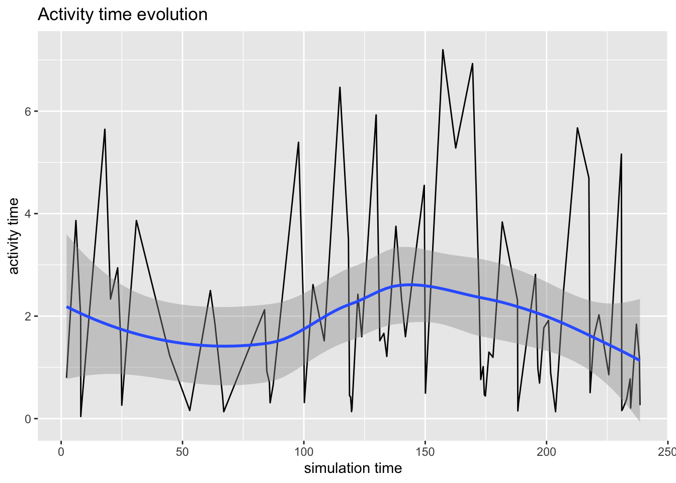
plot(arrivals, metric = "waiting_time")`geom_smooth()` using method = 'loess' and formula = 'y ~ x'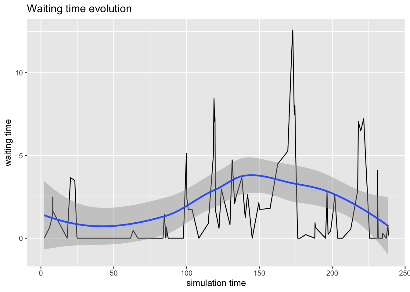
plot(arrivals, metric = "flow_time")`geom_smooth()` using method = 'loess' and formula = 'y ~ x'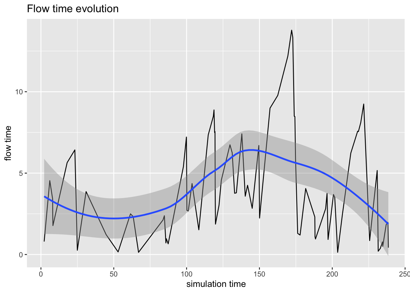
5 Conclusion
- Simmer is a powerful tool for building and simulating discrete event systems
- Once we can define the components and dynamics we can build a simulation
- We can visualize the model we’ve built to make sure it matches our expectations
- All the details are handled for us
6 Next Steps
- Working with our own distributions
- More complex systems such as:
- different paths
- different servers
- different customers