#6 Custom Distributions & Reliability (NJT)

14:540:384: Simulation Models in IE (Spring 2025)

Author

Affiliation

Daniel Moore

Rutgers University

Published

2025-02-26

Questions

Review

Shown why we need simulations and a few practical examples
Discussed where distributions come from, how to get them and how to use them
Shown how to manipulate data and create visualizations
Demonstrated two coding patterns for simulations
Shown how simmer provides nautral abstractions to build models and handle the simulation part for us

1 Learning Objectives

Model a system’s reliability
Fit distributions to data
Implement a custom distribution
Simulate the failures and evaluate the reliabilty

2 Problem

fictional

New Jersey Transit is pushing Amtrak to increase its reliability from Trenton to Newark Penn Station. There is one specific track outside of Trenton which has a problematic spot due to the hydrology and subgrade geology which results in a few different failures. Any one failure will result in speed restrictions and slow operations, but the track will remain operational and the fault will not be addressed. If a second failure occurs, the track will be shut down and all faults will be repaired. Because these are frequent problems the maintenance crews are well prepared to repair the system overnight.

One option on the table is to shut down the track for a period of three months to make significant subgrade improvements which would effectively eliminate these failures. The chief would like to evaluate the costs associated with the current, intermittent repairs and costs to the systems vs. the cost to make improvements and the prolonged shutdown. She has asked you to estimate the number of failures to expect in 10 years, provide estimated reilability vs. time. Additionally, she would like to know the probability that the time between two failures is more than 6 months and the 25th-percentile system failure time.

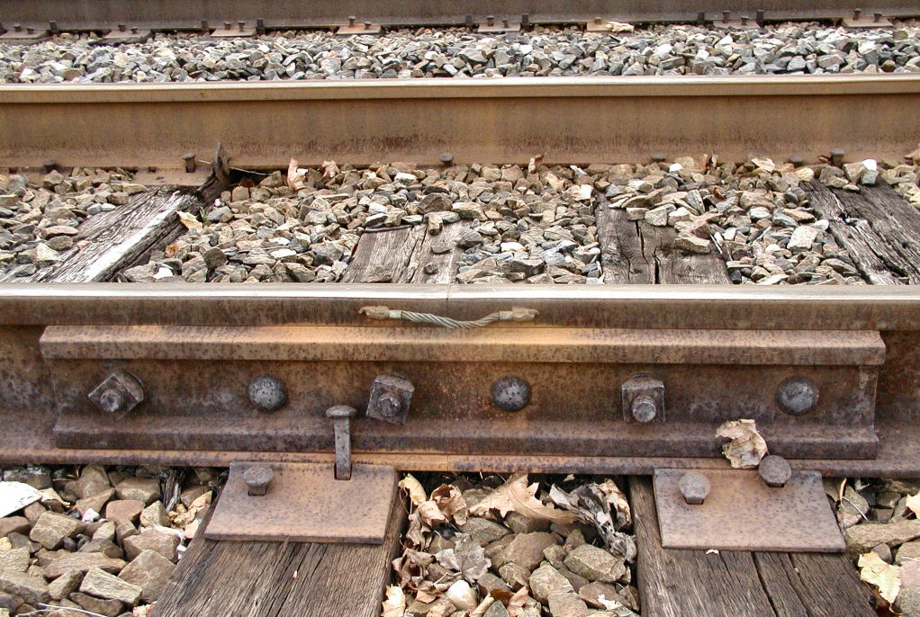
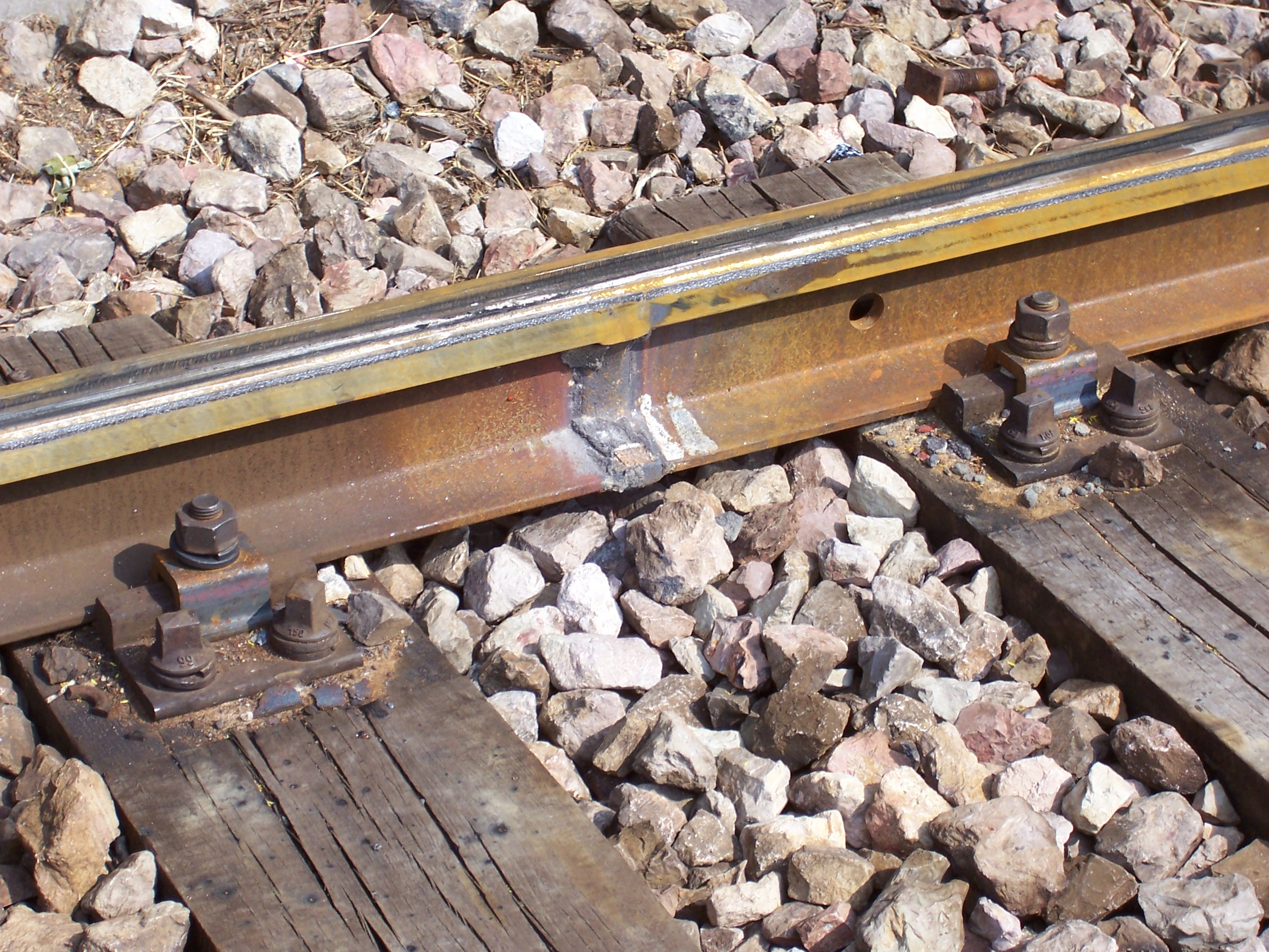
2.1 Failure Modes

It is assumed that the modes of failure are independent. The three failures at this spot are:

Continuous Welded Rail (CWR) failure: The entire Northeast Corridor is a CWR system meaning each rail is welded to the next. The rail welds are considered ok if at most one out of four welds have failed. (The four welds being the two at both ends of both the left and rigth rails). Individual welds have failed more frequently here than most rail sections. An initial estimate is that they fail at exponentially distributed times of four times per year.
Railroad Ties. Timber railroad ties are used in this area because of the frequent overnight repairs. However they also wear out faster as they are susceptible to rot. The ties are replaced as needed. As a system of ~20 ties per section of rail, it is taken that the ties will degrade to the point of failure at exponentially distributed times with an average of three times per year in this location.
“Mud-pumping”: This occurs from the vibrations of the train over an area of track which has poor drainage. Over time, the ballast under the tracks gets compressed and pushed away until the rail and ties are “floating” above the ballast as a beam. This failure is progressive once it begins. However, the time between it beginning is not well studied. Data from the field has been collected and recent studies have suggested that the (Generalized Gamma Distribution)[https://en.wikipedia.org/wiki/Generalized_gamma_distribution] might offer an appropriate failure time distribution model.

2.2 Failure Mode (cont.)

3 Modeling this System

Let’s draw a picture
Explain your concept of the problem
How does this system fail?
How will you simulate it?

3.1 Load Packages

library(tidyverse)
library(knitr)
library(fitdistrplus)

3.2 Failure Time Distributions

Each weld fails at \(Exp\sim(4/year)\)
We need the time until how many welds fail?
How to model this?

n_failures <- 2
lambda_cwr <- 365/4

cwr <- function(n=1) {
  rgamma(n, n_failures, rate=1/lambda_cwr)
}

The section of rail has an accepted exponentially distriubted failure times of 3/year

lambda_rrt <- 365/3

rrt <- function(n=1) {
  rexp(n, rate=1/lambda_rrt)
}

degenerative failure
failures are correlated to significant weather events, but these are also random
once a fault begins, it progresses at an accelerated rate to failure
we’ve been directed to compare a Generalized Gamma Distribution to other fits
we’ll compare it against our trusty Weibull distribution

Two Distributions

Generalized Gamma pdf is given by Equation 1:

\[ f(t; \theta, \kappa, \delta) = \frac{(\delta/\theta^\kappa)t^{\kappa-1} e^{-(t/\theta)^\delta}}{\Gamma(\kappa/\delta)} \tag{1}\]

Scale Parameter: \(\theta\)
Shape Parameter: \(\kappa\)
Power Parameter: \(\delta\)

And Weibull pdf is given by Equation 2:

\[ f(t; k, \lambda) = \frac{k}{\lambda}\left( \frac{t}{\lambda} \right)^{k-1} \tag{2}\]

Scale parameter: \(\lambda\)
Shape parameter: \(k\)

4 Fitting the Mud-Pumping distribution

How do you want to fit the specified distribution to the provided data?

fitdistrplus overview “Distributions not found in any package must be implemented by the user as d, p, q functions.”

4.1 Obtain Data

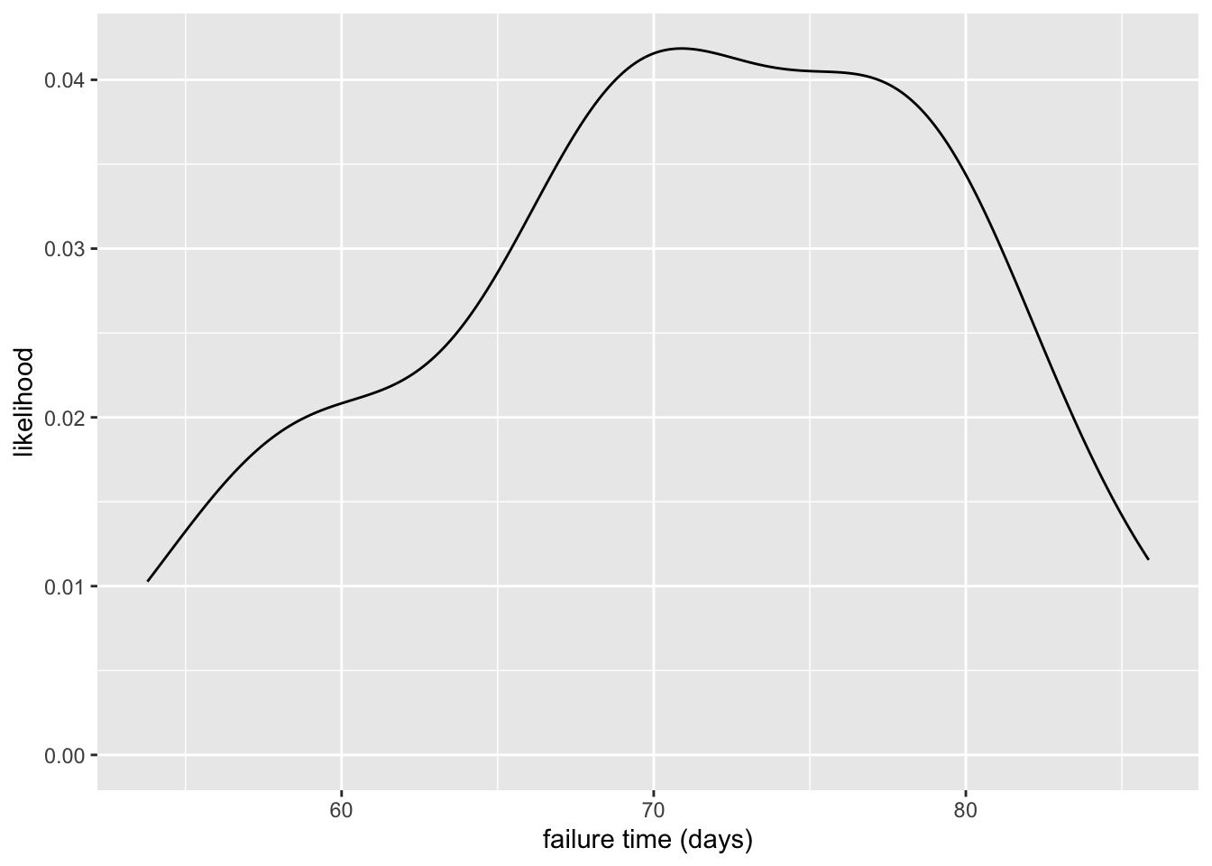
create a tibble around read_csv function to load the data as a tibble
plotting a histogram and and a “smoothed” density plot for basic data inspection

mp_ft <- tibble(read_csv("mud-pumping-failure-times.csv"))

mp_ft |> ggplot(aes(x = failure_times_days)) +
  geom_histogram() +
  labs(
    x = "failure time (days)",
    y = "count"
  )

mp_ft |> ggplot(aes(x = failure_times_days)) +
  geom_density() +
  labs(
    x = "failure time (days)",
    y = "likelihood"
  )

4.2 Implement Method

Documentation indicates we need to provide:

probability density function d<functionname>
quantile function q<functionname>
cumulative distribution function p<functionname>

Our function name will be ggamma so we need dggamma, qggamma, pggamma

Must follow the same argument names as other distributions. For example see the normal distribution functions:

dnorm(x, mean = 0, sd = 1, log = FALSE)
pnorm(q, mean = 0, sd = 1, lower.tail = TRUE, log.p = FALSE)
qnorm(p, mean = 0, sd = 1, lower.tail = TRUE, log.p = FALSE)
rnorm(n, mean = 0, sd = 1)

\[ \log(f(x) = \log(\delta) - \kappa \log(\theta) - \log \Gamma\left(\frac{\kappa}{\delta}\right) + (\kappa - 1) \log(x) - \left(\frac{x}{\theta}\right)^\delta \]

# Generalized Gamma PDF
# Generalized Gamma PDF
dggamma <- function(x, theta, kappa, delta, log = FALSE) {
  # Handle zero-length input
  if (length(x) == 0) return(numeric(0))
  
  # Compute log-density
  val <- log(delta) - kappa * log(theta) - lgamma(kappa / delta) + 
         (kappa - 1) * log(x) - (x / theta)^delta
  
  if (log) return(val) else return(exp(val))
}

# Generalized Gamma CDF
pggamma <- function(q, theta, kappa, delta, log.p = FALSE) {
  # Handle zero-length input
  if (length(q) == 0) return(numeric(0))
  
  # Corrected transformation
  val <- pgamma((q / theta)^delta, shape = kappa / delta, scale = 1, log.p = log.p)
  
  return(val)
}

# Generalized Gamma Quantile Function
qggamma <- function(p, theta, kappa, delta) {
  # Handle zero-length input
  if (length(p) == 0) return(numeric(0))
  
  # Compute quantile
  out <- theta * (qgamma(p, shape = kappa / delta, scale = 1)^(1 / delta))
  return(out)
}

4.3 Fit the Distributions

theta_start <- mean(mp_ft$failure_times_days)  # Scale estimate
kappa_start <- (mean(mp_ft$failure_times_days)^2) / var(mp_ft$failure_times_days)  # Shape estimate
delta_start <- 1  # Start with 1 and optimize


f_ggamma <- fitdist(
  mp_ft$failure_times_days, "ggamma",
  start = list(
    theta = theta_start,
    kappa = kappa_start,
    delta = delta_start)
  )

Warning in cov2cor(varcovar): diag(V) had non-positive or NA entries; the
non-finite result may be dubious

Warning in sqrt(diag(varcovar)): NaNs produced

f_weibull <- fitdist(
  mp_ft$failure_times_days,
  "weibull"
)

plot.legend <- c("Generalized Gamma", "Weibull")

4.4 Plot Results

Density Comparison

denscomp(list(f_ggamma, f_weibull), legendtext = plot.legend)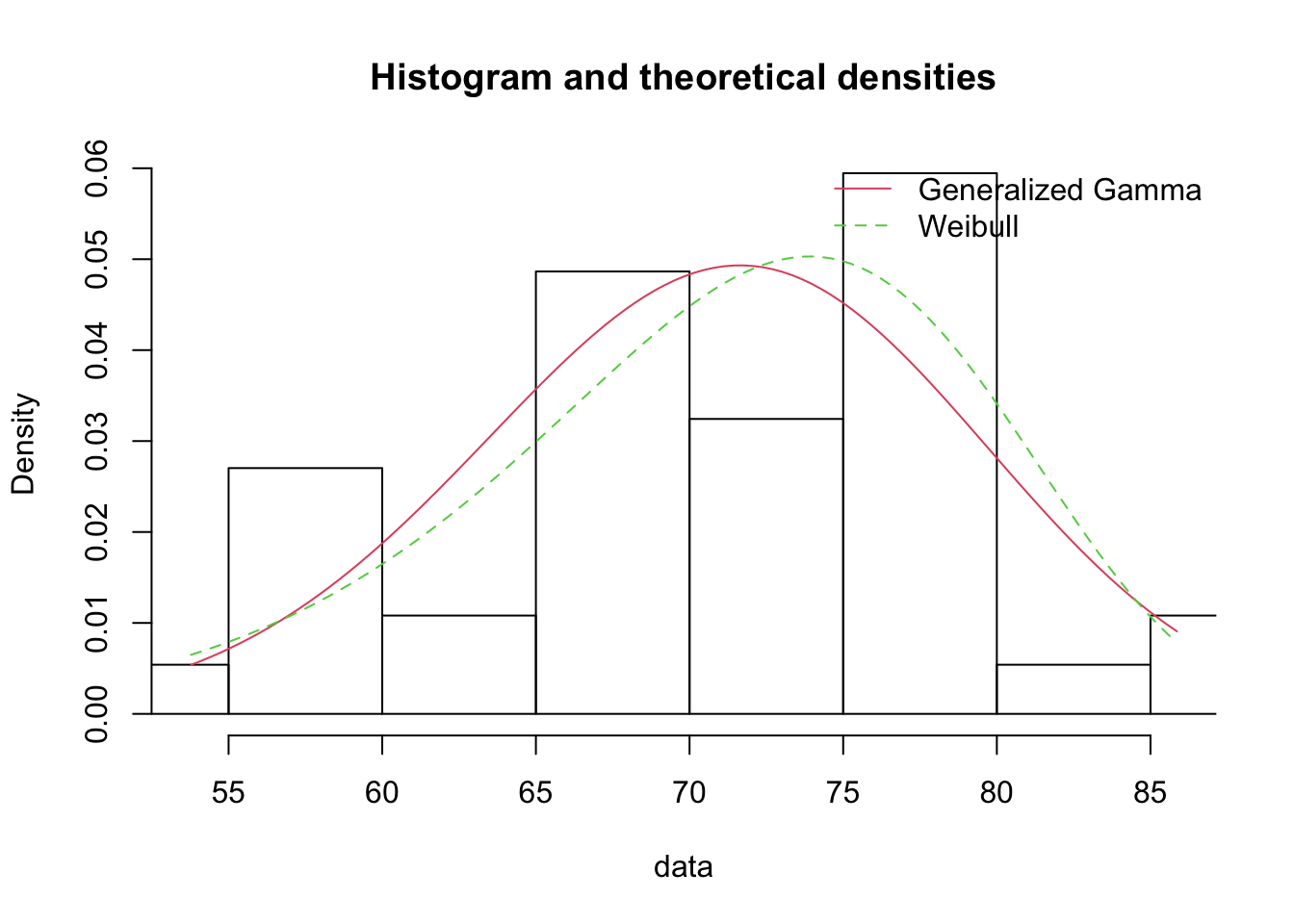

Quantile-Quantile Comparison

qqcomp(list(f_ggamma, f_weibull), legendtext = plot.legend)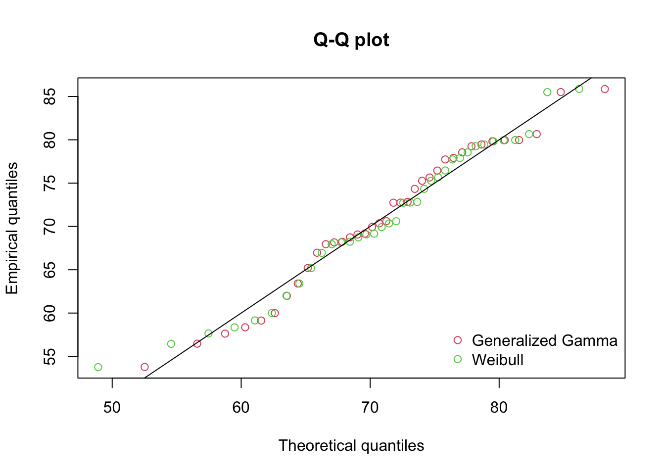

CDF Comparison

cdfcomp(list(f_ggamma, f_weibull), legendtext = plot.legend)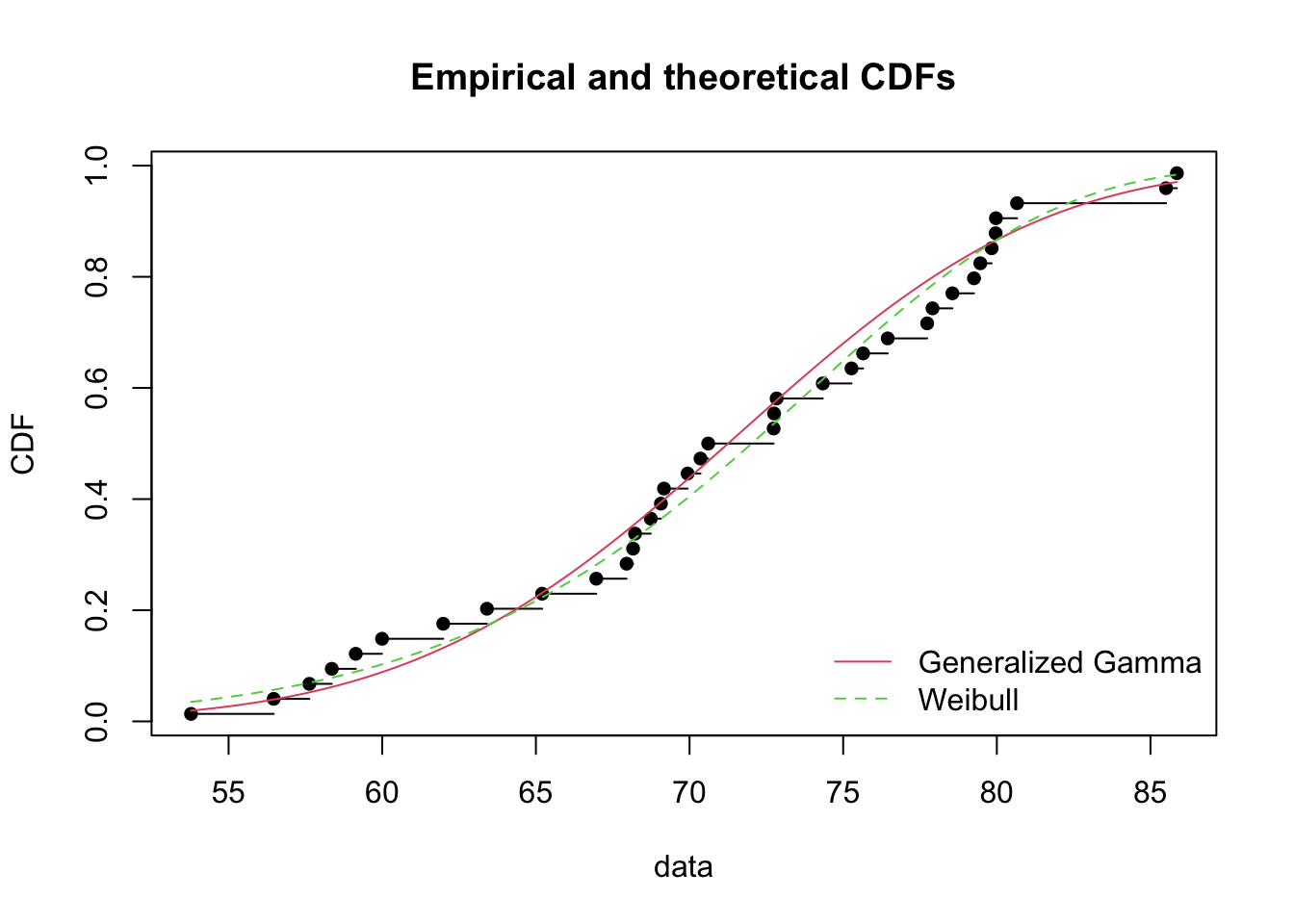

Probability-Probability Comparison

ppcomp(list(f_ggamma, f_weibull), legendtext = plot.legend)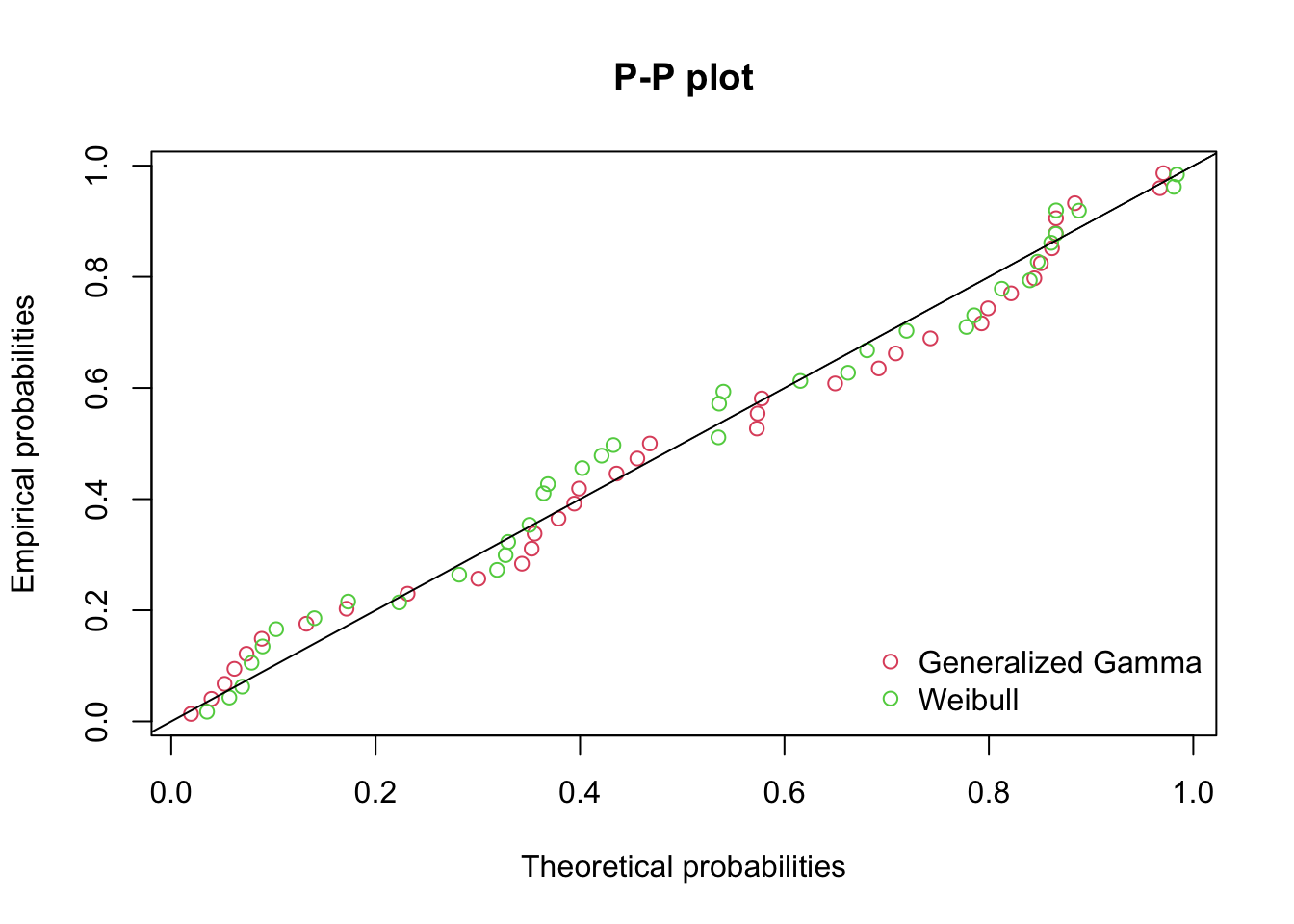

4.5 Select Evaluation Criteron

These diagnostic plots are helpful, but we need something more defensible

Various criteria found in course notes.

MSE, SSE, Likelihood, AIC, BIC all provided by fitdistrplus.
Pham’s Criteron (PC): Increase slightly the penalty each time adding parameters in the model when there is too small a sample.

\[ PC = \left( \frac{n-k}{2} \right) \log \left(\frac{SSE}{n} \right) + k \left( \frac{n-1}{n-k} \right) \]

PC <- function(SSE, n, k) {
  ((n-k) / 2) * log(SSE/n) * k * ((n-1) / (n-k))
}

Number of samples, \(n\)
Number of parameters, \(k\)
Sum of Squared Error, \(SSE\)

Predicted Density Values

# n is number of observations
n <- length(mp_ft$failure_times_days)
# k is number of parameters
k_ggamma <- length(f_ggamma$estimate)
k_weibull <- length(f_weibull$estimate)

dens_ggamma_pred <- dggamma(
  mp_ft$failure_times_days,
  theta = f_ggamma$estimate["theta"],
  kappa = f_ggamma$estimate["kappa"],
  delta = f_ggamma$estimate["delta"]
)

dens_weibull_pred <- dweibull(
  mp_ft$failure_times_days,
  shape = f_weibull$estimate["shape"],
  scale = f_weibull$estimate["scale"]
)

Comparison to Emprical Densities

# Compute empirical density
dens_emp <- density(mp_ft$failure_times_days)

# Interpolate empirical density to match predicted values
empirical_vals <- approx(dens_emp$x, dens_emp$y, xout = mp_ft$failure_times_days, rule = 2)$y


# Compute Sum of Squared Errors (SSE) for generalized gamma
sse_ggamma <- sum((empirical_vals - dens_ggamma_pred)^2)
f_ggamma$SSE <- sse_ggamma

# Compute Sum of Squared Errors (SSE) for Weibull
sse_weibull <- sum((empirical_vals - dens_weibull_pred)^2)
f_weibull$SSE <- sse_weibull

# Evaluate PC for the two distributions
f_ggamma$PC <- PC(sse_ggamma, n, k_ggamma)
f_weibull$PC <- PC(sse_weibull, n, k_weibull)

fitted_distributins <- list(f_ggamma, f_weibull)

summary_table <- sapply(fitted_distributins, function(fit) {
  c(
    "Number of Parameters" = as.integer(length(fit$estimate)),  # Number of parameters
    "Log-Likelihood" = fit$loglik,                # Log-likelihood
    "AIC" = fit$aic,                              # Akaike Information Criterion
    "BIC" = fit$bic,                              # Bayesian Information Criterion
    "SSE" = fit$SSE,           # Sum of Squared Error
    "PC" = fit$PC            # Pham's Criteron
  )
})

colnames(summary_table) <- c("Gen Gamma", "Weibull") 

kable(summary_table)

Goodness of Fit Measures
	Gen Gamma	Weibull
Number of Parameters	3.0000000	2.0000000
Log-Likelihood	-130.0411499	-129.8294174
AIC	266.0822998	263.6588348
BIC	270.9150535	266.8806706
SSE	0.0011993	0.0008403
PC	-558.1960808	-384.9360366

Based on these results, we will opt for the Weibull distribution as it has a prefereable AIC, BIC, and SSE while the Log-Likelihoods were basically the same. While Pham’s criteria was better for the Generalized Gamma, we know that the Weibull is just a special case of the Genearlized Gamma and we prefer the simpler model when other metrics give ambiguous options.

mp <- function(n=1) {
  rweibull(n, shape=f_weibull$estimate["shape"], scale=f_weibull$estimate["scale"])
}

5 Simulation

5.1 Options

While-loop
Sample batches of failure times
Use simmer

5.2 Implementation

we have our distributions
we can sample a set of each one and take the 2nd failure time as the system failure time
putting this in a table we can easily obtain (simulated) empirical results to the questions asked by the boss

Running the Smulation

# number of scenarios
n <- 10000

rail_sim <- tibble(
  scenario = 1:n,
  CWR = cwr(n),
  RR = rrt(n),
  MP = mp(n)
)

rail_sim <- rail_sim |>
  mutate(
    # select only the last 3 columns (not "scenario")
    System = apply(rail_sim[,2:4], 1, function(row) {
      # sort the values
      sorted_vals <- sort(row, decreasing = TRUE)
      # select the second largest
      sorted_vals[2]
    })
  )

kable(head(rail_sim))

scenario	CWR	RR	MP	System
1	115.90712	123.59601	76.70320	115.90712
2	178.50519	94.88911	79.24958	94.88911
3	160.06414	87.77702	67.08204	87.77702
4	122.72799	237.35260	73.92576	122.72799
5	56.74571	187.26485	58.12133	58.12133
6	434.67060	170.44813	77.43264	170.44813

Pivot Data For Plotting

rail_sim_long <- rail_sim |> pivot_longer(
  cols = -scenario,
  names_to = "Failure Type",
  values_to = "Failure Time"
)

kable(head(rail_sim_long))

scenario	Failure Type	Failure Time
1	CWR	115.90712
1	RR	123.59601
1	MP	76.70320
1	System	115.90712
2	CWR	178.50519
2	RR	94.88911

rail_sim_long |> ggplot(aes(x=`Failure Time`, color=`Failure Type`)) +
  stat_ecdf()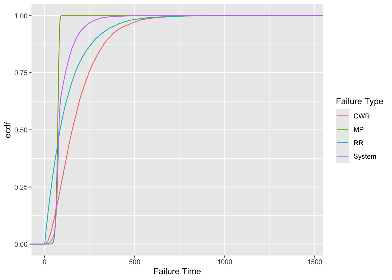

5.3 Required Metrics

# simply averaging the failure time of the system
mean_sys_ft <- mean(rail_sim$System)

# applying that to 10 years
number_fail_10yrs <- 10*365 / mean_sys_ft

# creating an empricial cumulative distribution function of the system failures
sys_ecdf <- ecdf(rail_sim$System)

# the probability of a failure being MORE than 180 days is 1 - ecdf(180)
p_6month <- 1 - sys_ecdf(180)

sys_ft_25thpercentile <- quantile(sys_ecdf, .25)

From the simulation:

The average failure time is 101.17 days.
This will result in ~37 failures in 10 years.
The probability of a failure occurring after more than 6 months is 9.3%.
The 25th percentile system failure time is 69.9 days.

5.4 Reliability Estimation

\(F(t)\) represents the probability of a failure occuring before time \(t\).
Reliability \(R(t)\) is the probability the system is functioning at time, \(t\).

\[ R(t) = 1 - F(t) \]

# simply create a function which is 1 - the system ecdf computed at that time
R_sys <- function(t) {
  1 - sys_ecdf(t)
}

# create a table 
sys_rel_table <- tibble(
  days = 0:(1.5*365),
  Reliability = R_sys(days)
)

sys_rel_table |> ggplot(aes(x=days, y=Reliability)) +
  geom_line()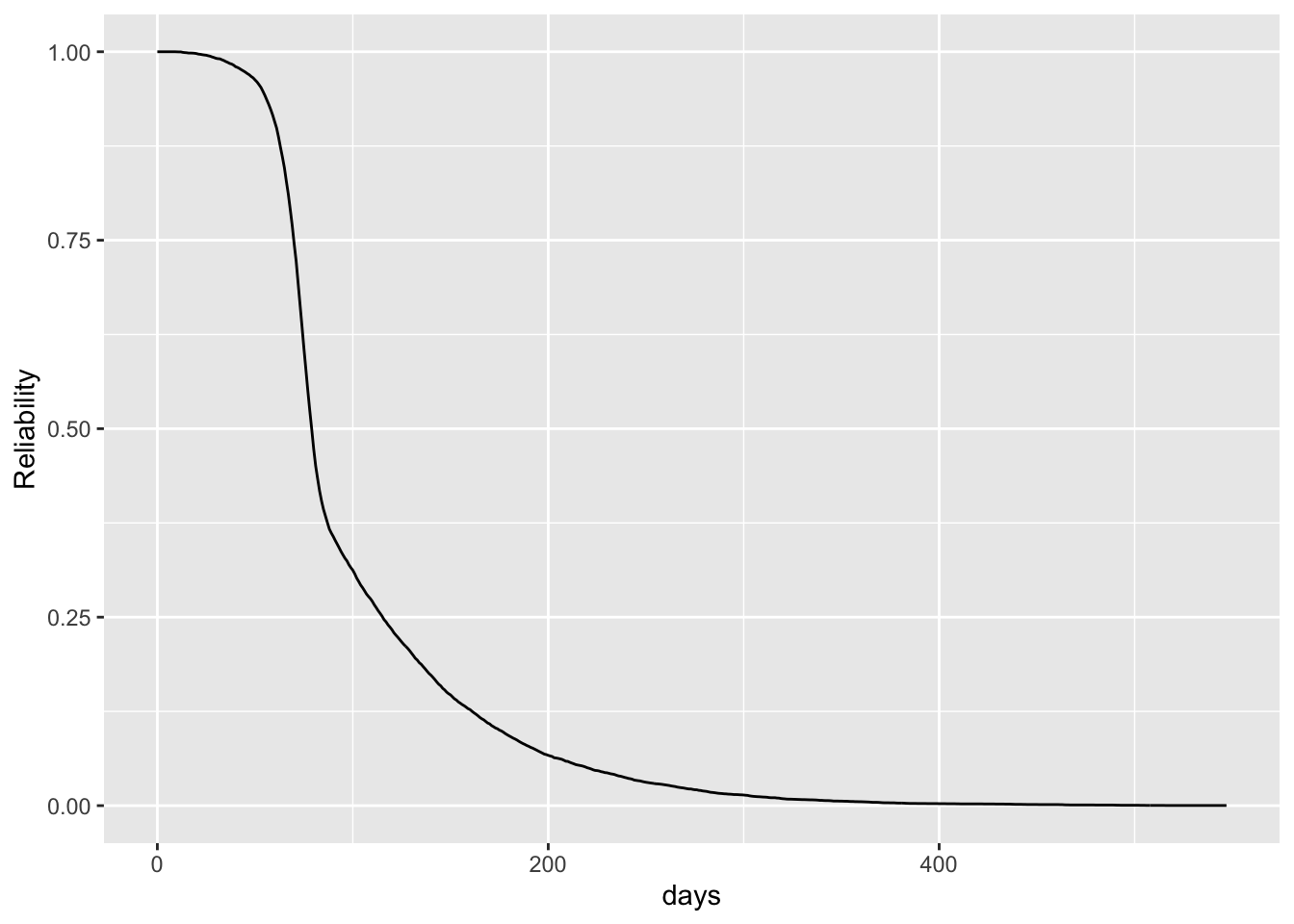

This is the estimated relability for the system
It represents that from any given repair time, this is the probability it will be functioning \(x\) days from then.

6 Conclusion

Recap

Parsed a complex problem into a simple framework
Identified how appropriate distributions should be selected
Demonstrated how to implement an “out-of-library” distribution
Fit distributions to the data
Built the model
Ran simulation and extracted results

Future Considerations

Test how our parameter estimates change the reliability curve
Consider more complex system failure such as an interaction amongst the failure mechanisms
Incorporate more distributions
Ultimately a different entity will use the information provided to Go/No-Go major repairs